Fast [Few-Single Step] Flow Matching

September 12, 2025

Flow matching is the most exciting, powerful and overall coolest successor of classical diffusion for generative tasks. Now powering SOTA image and video models like Stable Diffusion 3.5, FLUX.1 Kontext, and Wan. Either for the entire model or just a little tiny head, flow matching is now everywhere: world models, robotics, speech, RL.

Its simplicity makes the technique very compelling. If you wish to understand it, I have a guide on flow matching that gives a gentle introduction to the method! (it's hopefully done by the time you're reading this).

Here we'll explore just how far flow matching can go. Getting good results out of [few-single] steps is, practically, a significant challenge: it allows for faster, cheaper inference. Philosophically (though practical too really), there's an even more interesting question: is a single diffusion step still diffusion? We'll explore some techniques today and get closer to an answer.

Each method has a TLDR with joyful visualizations at the top. Skip the implementation if you just want the ideas

The Problem

The fundamental limitation of [few-one] step generation is directional ambiguity: at any noisy point there are multiple plausible data points that the model could map to, making the velocity field inherently uncertain. This shows as mode averaging, where models simply point toward dataset means rather than committing to a specific output.

What is mode averaging?

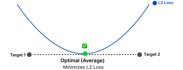
When training a neural network using L2 loss (mean squared error, shown below), it learns to predict averages. Why? Because the average minimizes squared distances to all possible outputs.

$\mathcal{L} = \mathbb{E}_{x,y}\left[\|f(x) - y\|^2\right]$

Think about it geometrically. If you have two points and need to pick one location that minimizes the squared distance to both, you'd pick the point exactly in the middle.

L2 Loss Geometric Intuition

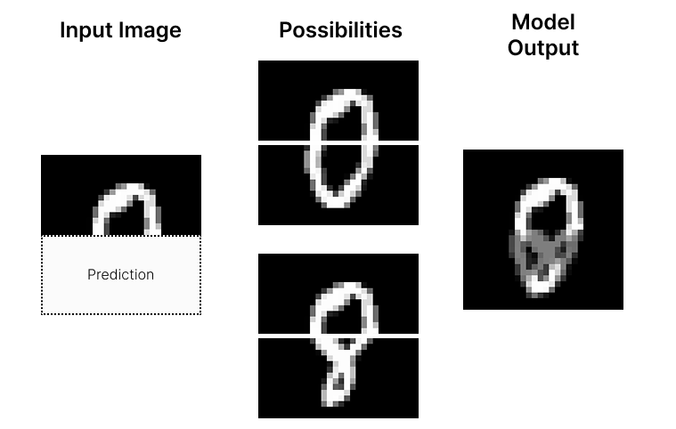
Now magine training a model to predict the bottom half of a hand written digit: give the top section as input, predict the bottom half. We then show it a rounded top as input. According to its training data, this could be either an 8 or a 0! Since it was trained with L2 loss, it will predict the average of both completions, a blurry mess.

MNIST Mode Averaging Example

This averagining behavior does make sense in some cases. Imagine now a model that outputs class probabilities based on images. If given a picture of both a cat and a dog, the output is correclty 1/2 dog, 1/2 cat!

Cat-Dog Mode Averaging Example

You see how this is mathematically optimal for the loss, but often meaningless for generative tasks where we want a specific output, not a blend.

The same problem affects flow matching. Just like our hand written digit model averages between 8 and 0, a single step in a standard flow model averages between all possible paths. Below we show this with a simple 2D example: a source distribution flowing to two separate target modes. The single-step prediction lands right in the middle, mode averaging again!

Single-Step Flow Matching

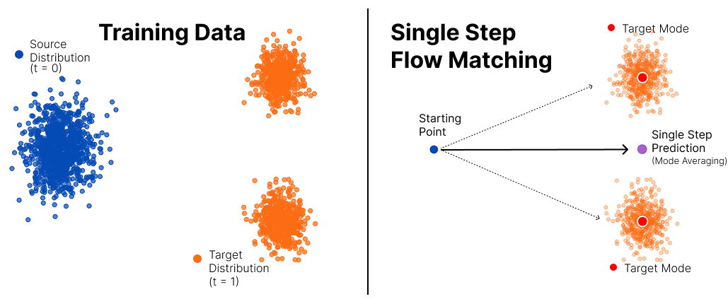
Just to drive home the idea, here's an example following a real model trained using standard flow matching. We have both the original and target distributions and the trajectories follow different step sizes. As you can see, the single step goes to the average!

Single-Step Flow Matching

Standard Flow Matching

Baseline Model

In order to understand everything properly I think it's worth it to show the simplest 'toy' example and them compare where these new few-step improvements come in, both comparing the code and the resulting visualizations.

Code

Here's the standard flow matching model we'll use as our baseline (4 linear layers, 3 ReLu activation layers):

class VectorFieldNN(nn.Module):
    def __init__(self, hidden_size=180):
        super().__init__()
        self.net = nn.Sequential(
            nn.Linear(3, hidden_size),
            nn.ReLU(),
            nn.Linear(hidden_size, hidden_size),
            nn.ReLU(),
            nn.Linear(hidden_size, hidden_size),
            nn.ReLU(),
            nn.Linear(hidden_size, 2),
        )

    def forward(self, x, t):
        inp = torch.cat([x, t], dim=1)  # (batch, 3)
        return self.net(inp)

And here's the documented training code for standard flow matching that we'll use as our baseline:

def train_standard_flow(model, num_epochs, batch_size, optimizer, device,
                        p_init_choice='gaussian', p_data_choice='checkerboard'):
    criterion = nn.MSELoss()
    loss_history = []

    for epoch in range(num_epochs):
        # Sample from source and target distributions
        x0 = sample_distribution(p_init_choice, batch_size, device)
        x1 = sample_distribution(p_data_choice, batch_size, device)

        # Sample random time
        t = torch.rand(batch_size, 1).to(device)

        # Linear interpolation
        x = (1 - t) * x0 + t * x1

        # Target constant velocity along linear path
        target = x1 - x0

        # Forward pass
        pred = model(x, t)

        # Loss
        loss = criterion(pred, target)

        # Backward pass
        optimizer.zero_grad()
        loss.backward()
        optimizer.step()

        loss_history.append(loss.item())

        # Logging
        if epoch % (num_epochs // 10) == 0:
            print(f"  Standard Flow - Epoch {epoch}/{num_epochs} - Loss: {loss.item():.4f}")

    return loss_history

Results

Here's a visualization of standard flow matching going from one toy distribution to another. Each row shows a different number of steps (1, 2, 4, 8), and each column shows snapshots at different times from t=0 to t=1. As you can see, the results for few-step generation are very messy!

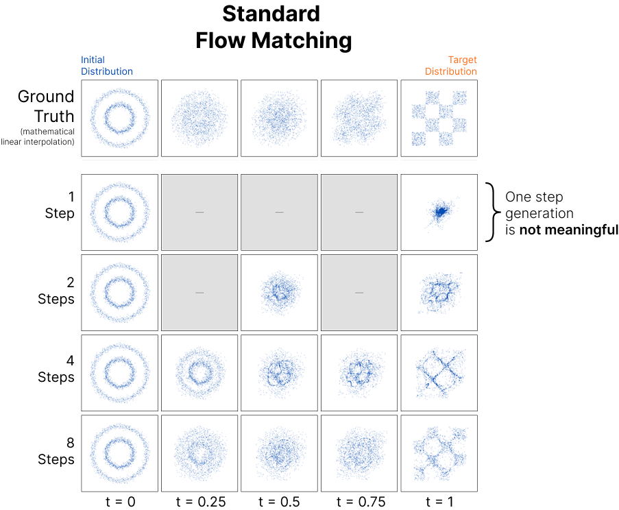
Standard flow matching visualization

The toy example shows the concept clearly. We also trained a full, real, model to see how flow matching performs on a realistic dataset.

Results from a DiT-S model (12 layers, 384 hidden size, ~33M parameters) trained on CelebA (162k samples at 256×256 resolution) for 180,000 steps using AdamW (lr=1.5e-4, batch size 135) on an RTX 4090 (~20-25 hours).

Below are samples generated at different step counts:

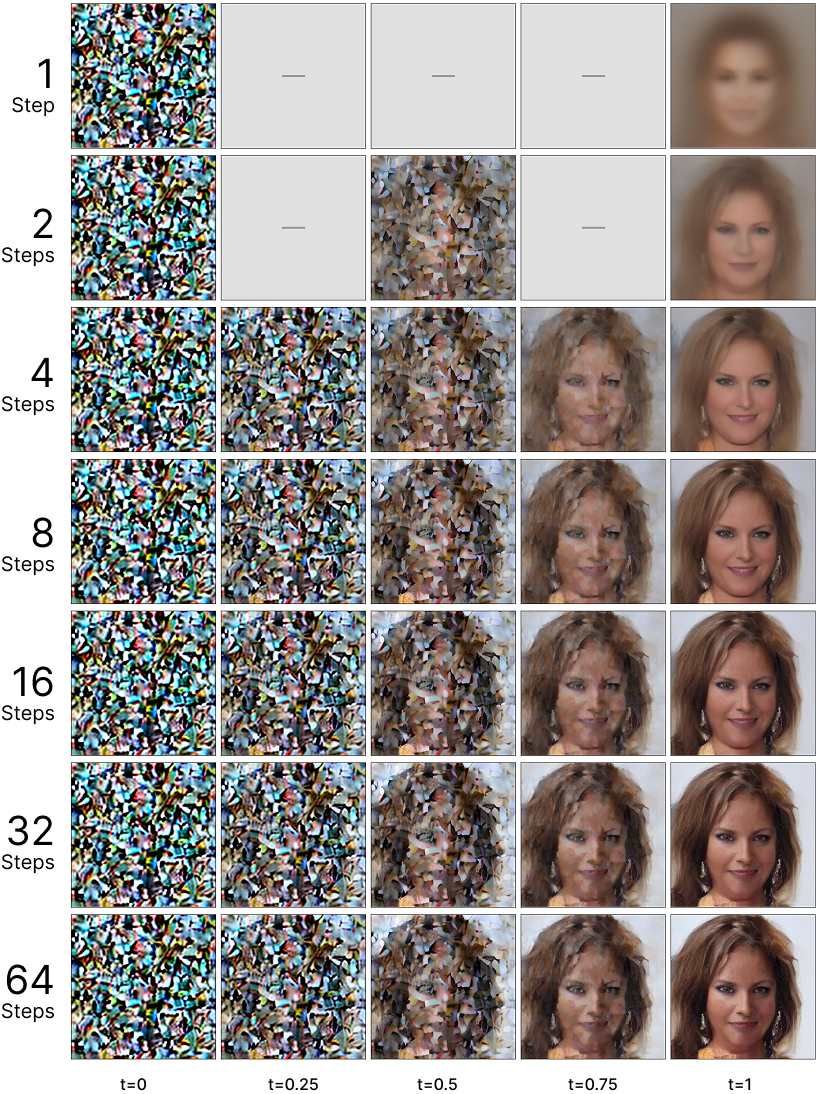
Standard Flow Matching CelebA Results

Average Human

[Few-Single] Step Flow Matching

Shortcut Models - [Paper]

TLDR:

We add a new parameter to the model: $dt$ , which encodes the step count. The model becomes $u_\theta(x_t, t, dt)$ .

Then we train it with a self-consistency trick: two small steps equal one big step. The model learns to adjust: a single step means a 'large' prediction, many steps means 'fine' predictions.

We train the model by doing 75% of normal, standard, flow matching and 25% of our special self-consistency trick. Single network, single training phase, no distillation needed.

The fundamental idea behind shortcut models is to condition the neural network not only on the current noise level (timestep t) but also on the desired step size (dt), allowing the model to accurately jump ahead in the generation process.

Standard flow matching:

u_\theta^{\text{standard}}(x_t, t)

Shortcut flow matching:

u_\theta^{\text{shortcut}}(x_t, t, dt)

(where $dt = \log_2(\text{steps})$ . We'll understand what $dt$ means in a moment.

The model learns to adjust its predictions based on how many steps it will take. One step? The model returns a large prediction. Many steps? It returns small, incremental predictions like standard flow matching.

How Shortcut Models Work

[0] Select Step Count

Remember: we added dt as an extra parameter to the model. This lets it adjust its predictions based on how many steps we plan to take.

Shortcut Model with dt parameter

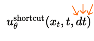
This is a parameter we give the model. We tell it to take 1, 2, 128 steps.

Now we need a way to 'encode' the step size. We said before that $dt = \log_2(\text{steps})$ . This means that if we give the model $dt = 0$ , we say 'take a single step'. If we give $dt = 1$ , 'take 2 steps'.

Why? This is a very sensible choice! Think about it, powers of two is a great way to encode the step we want the model to be conditioned on.

We can chose between: 1, 2, 4, etc steps. A sensible range.

If we used powers of 3, we would have something like 1, 3, 9, 27, 81. Which could work too but it's not as nicely spaced.

Log2 Step Encoding

We now choose dt_max (the maximum dt). This determines the range of step counts the model can handle. Therfore, if we want say {0, 2, 4} steps, the max step is 4, and dt_max would be 2. If we select dt_max to be 8, then our model would have powers of two steps until max steps of 256.

If we set $dt_{\text{max}} = 3$ , then $dt \in \{0, 1, 2, 3\}$ and the model can use step counts $\{1, 2, 4, 8\}$ .

During training, we randomly sample dt values from this range.

At the risk of being annoying, again:

if $dt_{\text{max}} = 7$ , then $dt \in \{0, 1, 2, 3, 4, 5, 6, 7\}$ , step_count = $\{1, 2, 4, 8, 16, 32, 64, 128\}$ .

[1] Sample Training Pairs

We simply sample from source/target distributions.

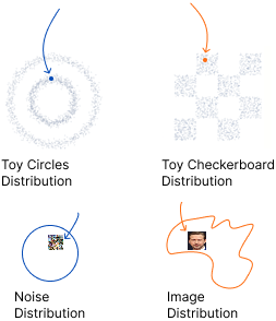
$x_0 \sim p_{\text{source}}, \quad x_1 \sim p_{\text{target}}$

Sample Training Paths

[2] Split Batch

Divide the batch between standard flow-matching and bootstrap training

Batch Split Diagram

[3] Flow-Matching Path

[75% of batch]

Sample random time t:

$t^{\text{flow}} \sim \text{Uniform}(0, 1)$

For standard flow matching, we use the finest resolution (dt = dt_max). The model predicts:

$u_\theta^{\text{flow}}(x_t^{\text{flow}}, t^{\text{flow}}, dt_{\text{max}})$

For example, if $dt_{\text{max}} = 7$ , standard flow matching will use dt = 7, which means 128 steps!

Interpolate:

$x_t^{\text{flow}} = (1-t^{\text{flow}})x_0 + t^{\text{flow}}x_1$

Target is constant velocity:

$v_{\text{target}}^{\text{flow}} = x_1 - x_0$

[4] Bootstrap Path

[25% of batch]

Sample random time:

$t^{\text{boot}} \sim \text{Uniform}(0, 1)$

Sample random coarse dt:

$dt^{\text{boot}} \sim \text{Uniform}\{0, 1, ..., dt_{\text{max}}-1\}$

$dt_{\text{fine}} = \min(dt^{\text{boot}} + 1, dt_{\text{max}})$

For example, if $dt_{\text{max}} = 7$ , we sample $dt^{\text{boot}} \in \{0, 1, 2, 3, 4, 5, 6\}$ and use $dt_{\text{fine}} \in \{1, 2, 3, 4, 5, 6, 7\}$ .

Say we sample $dt^{\text{boot}} = 0$ , then $dt_{\text{fine}} = 1$ . This means we use 1 coarse step and 2 fine steps

This is the trickiest part, please check carefully.

Interpolate:

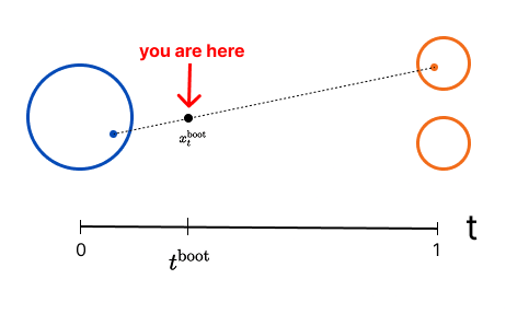
$x_t^{\text{boot}} = (1-t^{\text{boot}})x_0 + t^{\text{boot}}x_1$

Bootstrap Interpolation

Predict first fine velocity:

$v_1 = \text{model}(x_t^{\text{boot}}, t^{\text{boot}}, dt_{\text{fine}})$

We give the model the current position $x_t$ , time $t$ , and the fine dt to get back the velocity prediction at that point

Take first fine step:

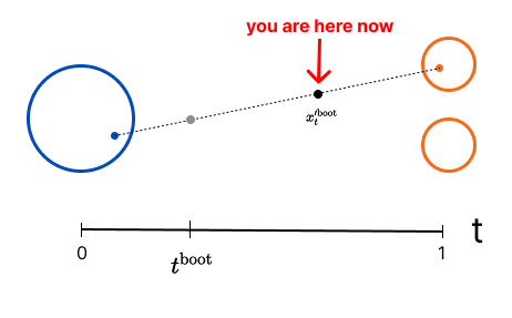
$x_t'^{\text{boot}} = x_t^{\text{boot}} + dt_{\text{fine}} \cdot v_1$

After First Fine Step

Since we know the velocity and our flow matching objective is linear interpolation, we can simply move forward. This is just Euler sampling

Predict second fine velocity:

$v_2 = \text{model}(x_t'^{\text{boot}}, t^{\text{boot}} + dt_{\text{fine}}, dt_{\text{fine}})$

Target is avg:

$v_{\text{target}}^{\text{boot}} = \frac{v_1 + v_2}{2}$

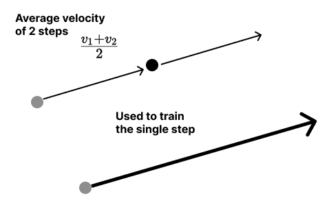
We predict $v_1$ and $v_2$ using the fine dt, but then we train the model to output their average when given the coarse dt. Say we sample $dt^{\text{boot}} = 0$ , then $dt_{\text{fine}} = 1$ . The model learns to match the quality of two 2-step predictions when asked for 1 step

We use two predictions from small steps to train the model on a single big step. It's self-distillation, think about it, the single step is the same as the average of two smaller ones

[5] Combine & Train

Concatenate bootstrap and flow-matching batches:

$x_t = [x_t^{\text{boot}}, x_t^{\text{flow}}], \quad t = [t^{\text{boot}}, t^{\text{flow}}], \quad v_{\text{target}} = [v_{\text{target}}^{\text{boot}}, v_{\text{target}}^{\text{flow}}]$

Calculate MSE:

$\mathcal{L} = \|\text{model}(x_t, t, dt) - v_{\text{target}}\|^2$

Code

Nothing crazy, we just define the model. Now we're taking in an extra condition, so we have 3 + 1 = 4 as input for the first linear layer.

class ShortcutNN(nn.Module):
    def __init__(self, hidden_size=180):
        super().__init__()

        self.net = nn.Sequential(
            # Change here!
            nn.Linear(4, hidden_size), # 3 + 1!
            #
            nn.ReLU(),
            nn.Linear(hidden_size, hidden_size),
            nn.ReLU(),
            nn.Linear(hidden_size, hidden_size),
            nn.ReLU(),
            nn.Linear(hidden_size, 2),
        )

    def forward(self, x, t, dt_base):
        # Normalize dt_base to [0, 1] range (assuming max is 3)
        dt_norm = dt_base / 3.0

        # Concatenate all inputs
        inp = torch.cat([x, t, dt_norm], dim=1)

        return self.net(inp)

Now for training.

Setup training, MSE loss (what we described at the top, remember?)

def train_shortcut_flow(model, num_epochs, batch_size, optimizer, device,
                        p_init_choice='gaussian', p_data_choice='checkerboard',
                        max_steps=8, bootstrap_ratio=0.25):

    criterion = nn.MSELoss()
    loss_history = []

[0] Select Step Count

Now calculate the sizes. We have a number of max steps, what are the maximum steps we can take? In this case 8, so dt_base = 3

    # Calculate sizes
    max_dt_base = int(np.log2(max_steps))  # 3 for 8 steps
    bootstrap_size = int(batch_size * bootstrap_ratio)  # 25% for bootstrap
    flow_size = batch_size - bootstrap_size  # 75% for standard flow matching

[1] Sample Training Pairs

We simply sample at first, just like normal flow matching, we get from our initial and target distributions.

    for epoch in range(num_epochs):
        # Sample from distributions
        x0_full = sample_distribution(p_init_choice, batch_size, device)
        x1_full = sample_distribution(p_data_choice, batch_size, device)

[2] Split Batch

First change! We split, we will use some of our samples for 'standard' flow matching and the others for our 'shortcut' objective!

        # Split for bootstrap and flow-matching
        x0_boot = x0_full[:bootstrap_size]
        x1_boot = x1_full[:bootstrap_size]
        x0_flow = x0_full[bootstrap_size:]
        x1_flow = x1_full[bootstrap_size:]

[3] Flow-Matching Path

Generate standard flow-matching targets.

        #
        # Flow-Matching Targets
        #

        # Sample random time t
        t_flow = torch.rand(flow_size, 1).to(device)

        # Use finest dt_base for flow-matching samples
        dt_base_flow = torch.full((flow_size, 1), max_dt_base, device=device)

        # Interpolate between x0 and x1
        x_t_flow = (1 - t_flow) * x0_flow + t_flow * x1_flow

        # Target is constant velocity
        v_target_flow = x1_flow - x0_flow

[4] Bootstrap Path

Generate bootstrap targets using two fine steps.

      #
      # Bootstrap Targets
      #

      # Sample random time t
      t_boot = torch.rand(bootstrap_size, 1).to(device)
      # Sample dt_base for coarse steps
      dt_base_boot = torch.randint(0, max_dt_base, (bootstrap_size, 1), device=device).float()

      # Use finer steps for bootstrap generation
      dt_base_finer = torch.clamp(dt_base_boot + 1, max=max_dt_base)

      # Calculate step sizes
      dt_coarse = 1.0 / (2 ** dt_base_boot)
      dt_fine = dt_coarse / 2

      # Interpolate between x0 and x1
      x_t_boot = (1 - t_boot) * x0_boot + t_boot * x1_boot

      # Generate bootstrap targets using two-step prediction
      with torch.no_grad():
          # First fine step
          v1 = model(x_t_boot, t_boot, dt_base_finer)

          # Take half step forward
          t2 = torch.clamp(t_boot + dt_fine, max=1.0)
          x_t2 = x_t_boot + dt_fine * v1

          # Second fine step
          v2 = model(x_t2, t2, dt_base_finer)

          # Average velocities for shortcut target
          v_target_boot = (v1 + v2) / 2

[5] Combine & Train

Combine both target types and train.

        #
        # Combine and Train
        #

        # Literally concatenate flow-matching and bootstrap
        # y = [bootstrap, flow_matching]
        x_t = torch.cat([x_t_boot, x_t_flow], dim=0)
        t = torch.cat([t_boot, t_flow], dim=0)
        dt_base = torch.cat([dt_base_boot, dt_base_flow], dim=0)
        v_target = torch.cat([v_target_boot, v_target_flow], dim=0)

        # Forward pass
        # We pass the concat tensors to the model
        # model( [boostrap_x, flow_matching_x],
        #   [bootstrap_t, flow_matching_t],
        #   [bootstrap_dt, flow_matching_dt])
        v_pred = model(x_t, t, dt_base)

        # Compute MSE loss on both bootstrap and flow-matching predictions
        loss = criterion(v_pred, v_target)

        # Backward pass
        optimizer.zero_grad()
        loss.backward()
        optimizer.step()

        loss_history.append(loss.item())

        # Log progress every 10% of training
        if epoch % (num_epochs // 10) == 0:
            print(f"  Shortcut - Epoch {epoch}/{num_epochs} - Loss: {loss.item():.4f}")

    return loss_history

Results

And here's how Shortcut Models perform:

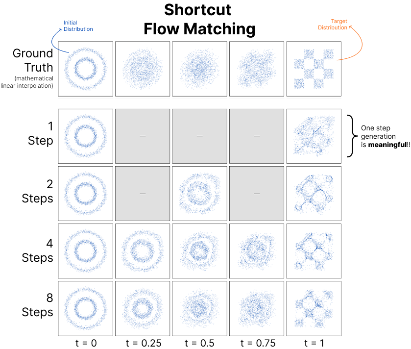
Shortcut flow matching visualization

Results from a DiT-S model (~33M parameters) trained on CelebA (256×256) for 180,000 steps with bootstrap ratio=0.25 (25%) and 128 denoise timesteps, using AdamW (lr=1.5e-4, batch size 135) on an RTX 4090 (~20-25 hours).

Below are samples generated at different step counts:

Shortcut Model Grid

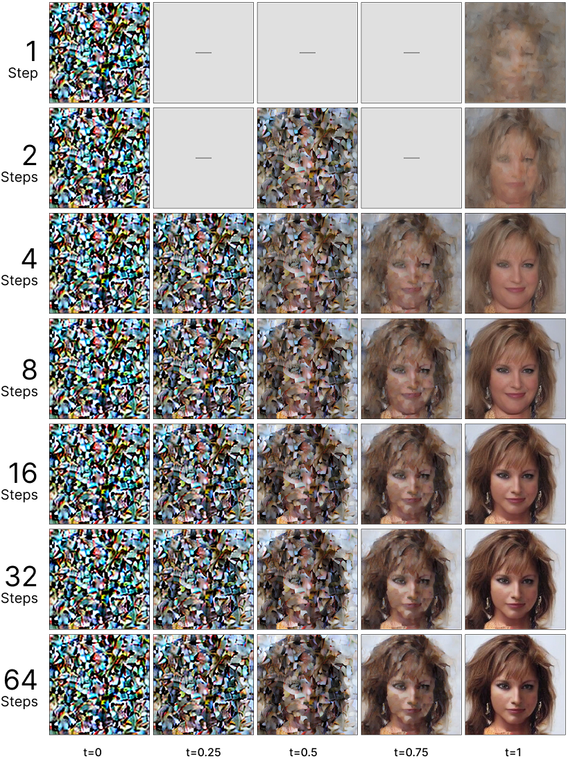
The one-step results might not look as exciting as you would expect, but you can actually see the difference. We're getting meaningful one-step generation unlike standard flow matching which simply averages the faces together and looks like a blob. This scales very well: the bigger the model, the longer the training, the better the single-step generation. Training was also extremely stable, and I didn't really have any problems.

The paper also found that standard flow matching itself improves with the Shortcut model, so even multi-step generation gets better which is interesting. It hasn't been explored much.

I have some other research on changing how we do step averaging. What happens if we use something other than linear interpolation? Also some fun multi-step inpainting models, but I won't share here because this is too long already.

MeanFlow - [Paper]

TLDR:

Instead of predicting instantaneous velocity, we train the model to predict average velocity over a time interval. We sample two time points (r, t) and use calculus to derive the target: the average equals the instantaneous velocity minus a derivative correction term computed via JVP.

No model architecture changes, just a modified training target with automatic differentiation. Single network, single training phase.

The results show how the model learns to denoise in a single step, gradually refining from noise to a coherent image.

Standard flow matching trains a model to predict instantaneous velocity $v(z_t, t)$ at each time point. MeanFlow trains the model to predict average velocity $u(z_t, r, t)$ over a time interval $[r, t]$ .

The average velocity is defined as displacement divided by time:

u = \frac{1}{t-r} \int_r^t v(\tau) \mathrm{d}\tau

Setting $(r, t) = (0, 1)$ gives the average velocity over the entire trajectory, which is the quantity needed for one-step sampling.

The MeanFlow Identity

By differentiating the definition of average velocity with respect to $t$ , we get the MeanFlow Identity:

MeanFlow Identity

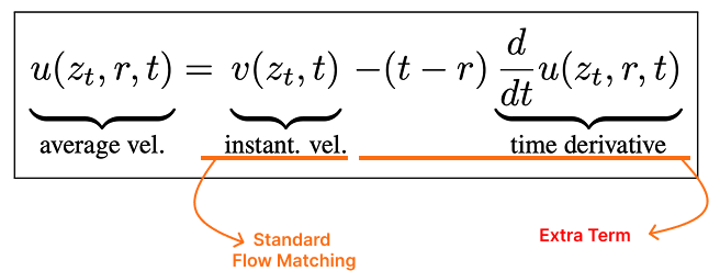
Average velocity equals instantaneous velocity (standard flow matching) minus an extra correction term.

The correction term involves the total derivative $\frac{d}{dt}u$ , which expands to:

$\frac{d}{dt}u(z_t, r, t) = v(z_t, t) \partial_z u + \partial_t u$

Remeber the total derivative:

$\begin{align*} \frac{d}{dt} u(z_t, r, t) &= \underbrace{\frac{\partial u}{\partial z_t} \cdot \frac{dz_t}{dt}}_{\text{spatial change as } z_t \text{ evolves}} + \underbrace{\frac{\partial u}{\partial r} \cdot \frac{dr}{dt}}_{\text{reference (zero!)}} + \underbrace{\frac{\partial u}{\partial t}}_{\text{explicit time dep.}} \end{align*}$

Now:

$\frac{dz_t}{dt} = v(z_t, t)$ : By definition! The velocity field tells us how $z_t$ changes with time along the flow.

$\frac{dr}{dt} = 0$ : The reference time $r$ is fixed, it doesn't change as we vary $t$ .

$\frac{\partial u}{\partial t}$ : The explicit time dependence of $u$ .

Therefore:

$\frac{d}{dt} u = \frac{\partial u}{\partial z_t} \cdot v(z_t, t) + \frac{\partial u}{\partial t} = v \cdot \partial_z u + \partial_t u$

This is a Jacobian-Vector Product (JVP) between the Jacobian $[\partial_z u, \partial_t u]$ and the tangent vector $[v, 1]$ .

Training Loss

We train a network $u_\theta$ to satisfy the MeanFlow Identity:

$\mathcal{L} = \mathbb{E}\|u_\theta(z_t, r, t) - \text{sg}(u_{\text{target}})\|^2$

where the target is:

$u_{\text{target}} = v_t - (t-r)(v_t \partial_z u_\theta + \partial_t u_\theta)$

Here $v_t = x_1 - x_0$ is the conditional velocity from standard flow matching, and $\text{sg}$ denotes stop-gradient to avoid double backpropagation.

Keep this in mind since this is what we'll aim to construct.

How MeanFlow Works

[0] Sample Time Interval

Sample two time points (r, t) where $r \leq t$ . We control how often $r = t$ (which reduces to standard flow matching) versus $r \neq t$ (which activates the JVP correction).

$r, t \sim \text{LogitNormal}(\mu, \sigma)$

For example, with 75% ratio of $r \neq t$ , we sample two independent times, sort them, then set $r = t$ for 25% of samples. Similar to shorcut models

[1] Sample Training Pairs

Sample from source and target distributions:

$x_0 \sim p_{\text{source}}, \quad x_1 \sim p_{\text{target}}$

Sample Training Paths

[2] Interpolate

Create the straight-line interpolation between source and target at time $t$ :

$z_t = (1-t)x_0 + t x_1$

Instantaneous velocity stays constant along this path:

$v_t = x_1 - x_0$

This is just standard flow matching, we now have $v_t$ .

$u_{\text{target}} = v_t - (t-r)(v_t \partial_z u_\theta + \partial_t u_\theta)$

[3] Compute JVP

Use automatic differentiation to compute:

$\frac{d}{dt}u_\theta(z_t, r, t) = v_t \partial_z u_\theta + \partial_t u_\theta$

This is computed via jvp(fn, (z, r, t), (v, 0, 1)) where the tangent vector is $(v_t, 0, 1)$ .

What JVP does:

Takes a function with multiple inputs: $f(x, y, z, \ldots)$

Takes a "direction vector": $(v_x, v_y, v_z, \ldots)$

Computes: $\frac{\partial f}{\partial x} \cdot v_x + \frac{\partial f}{\partial y} \cdot v_y + \frac{\partial f}{\partial z} \cdot v_z + \ldots$

In MeanFlow:

Function: $u(z_t, r, t)$ - the model

Direction: $(v_t, 0, 1)$ - flow direction for $z_t$ , nothing for $r$ , forward in time

Result: $\frac{du}{dt} = \frac{\partial u}{\partial z_t} \cdot v_t + \frac{\partial u}{\partial t}$ - this is $\frac{d}{dt} u$ , the total time derivative

This is extremely important to understand, it is basically the entire point of the paper. Let's explore deeper.

The main idea of JVP is to get the partial derivatives:

$\frac{\partial f}{\partial x}, \frac{\partial f}{\partial y}, \frac{\partial f}{\partial z}, ...$

In our case, we are doing this against our model, both for $z_t$ and $t$ . We're trying to get: $\frac{\partial u}{\partial z_t}, \frac{\partial u}{\partial t}$ (remember that the r is 0 so we don't care about that partial derivative).

What does it 'mean' for us to get these partial derivatives?

We're saying: for the function $u(z_t, r, t)$ , what happens if we move each parameter by a tiny amount.

So $\frac{\partial u}{\partial z_t}$ asks: what do we get out of $u(z_t + \epsilon, r, t)$ , where $\epsilon$ is a tiny tiny value.

Similarly, $\frac{\partial u}{\partial t}$ asks: what happens to the output of $u(z_t, r, t + \epsilon)$ , where $\epsilon$ is a tiny tiny value.

Conceptually this is like doing 2 forward passes: we 'run the model' with this extra tiny parameter, to see how the output would change with a tiny nudge in the input.

[Very important to say that we're not doing any weight changes here and also, technically, we're not doing 2 forward passes, it's done in one. This is just an intuition.]

[4] Compute Target

Apply the MeanFlow Identity:

$u_{\text{target}} = v_t - (t-r) \frac{d}{dt}u_\theta$

[5] Train

Minimize MSE loss:

$\mathcal{L} = \|u_\theta(z_t, r, t) - \text{sg}(u_{\text{target}})\|^2$

Code

We reuse the same backbone as standard flow matching; the only tweak is feeding both $r$ and $t$ as scalars (so in practice you simply extend the first linear layer’s input width by one to concatenate $r$ alongside $t$ ):

class FlowMatchingNN(nn.Module):
    def __init__(self, hidden_size=180):
        super().__init__()
        self.net = nn.Sequential(
            nn.Linear(3, hidden_size),  # x, t only (no extra dt parameter!)
            nn.ReLU(),
            nn.Linear(hidden_size, hidden_size),
            nn.ReLU(),
            nn.Linear(hidden_size, hidden_size),
            nn.ReLU(),
            nn.Linear(hidden_size, 2),
        )

    def forward(self, x, t):
        inp = torch.cat([x, t], dim=1)
        return self.net(inp)

When following the training loop below, concatenate $r$ as an additional scalar before the first layer (or equivalently wrap the network so it receives both $r$ and $t$ in one tensor) to match the $u_\theta(z, r, t)$ interface used in the paper.

The training loop implements the MeanFlow algorithm:

[0] Sample Time Interval

def sample_time_steps(batch_size, device, ratio_r_not_equal_t=0.75):
    # Sample from logit-normal distribution
    normal_samples = torch.randn(batch_size, 2, device=device)
    normal_samples = normal_samples * sigma + mu
    time_samples = torch.sigmoid(normal_samples)

    # Sort to ensure t > r
    sorted_samples, _ = torch.sort(time_samples, dim=1)
    r, t = sorted_samples[:, 0], sorted_samples[:, 1]

    # Control proportion of r=t samples
    fraction_equal = 1.0 - ratio_r_not_equal_t
    equal_mask = torch.rand(batch_size, device=device) < fraction_equal
    r = torch.where(equal_mask, t, r)

    return r, t

[1-2] Sample and Interpolate

# Sample training pairs
images = sample_batch(batch_size)  # x1
noises = torch.randn_like(images)  # x0 (noise)

# Sample time interval
r, t = sample_time_steps(batch_size, device)

# Interpolate
alpha_t = (1 - t).view(-1, 1, 1, 1)
sigma_t = t.view(-1, 1, 1, 1)
z_t = alpha_t * images + sigma_t * noises

# Instantaneous velocity
v_t = noises - images

[3] Compute JVP

from torch.func import jvp

def fn(z, cur_r, cur_t):
    return model(z, cur_r, cur_t)

# Compute model prediction and its derivative
primals = (z_t, r, t)
tangents = (v_t, torch.zeros_like(r), torch.ones_like(t))

u, dudt = jvp(fn, primals, tangents)

[4-5] Compute Target and Train

# Time difference
time_diff = (t - r).view(-1, 1, 1, 1)

# MeanFlow target
u_target = v_t - torch.clamp(time_diff, 0.0, 1.0) * dudt

# Loss with stop-gradient
error = u - u_target.detach()
loss = torch.mean(error ** 2)

# Standard backpropagation
optimizer.zero_grad()
loss.backward()
optimizer.step()

The key difference from standard flow matching is the JVP computation and the modified target. Everything else remains the same.

Results

There is something very significant to analyze before we show any results: we need to go back to the JVP computation.

We get to the problem of (non)smooth gradients.

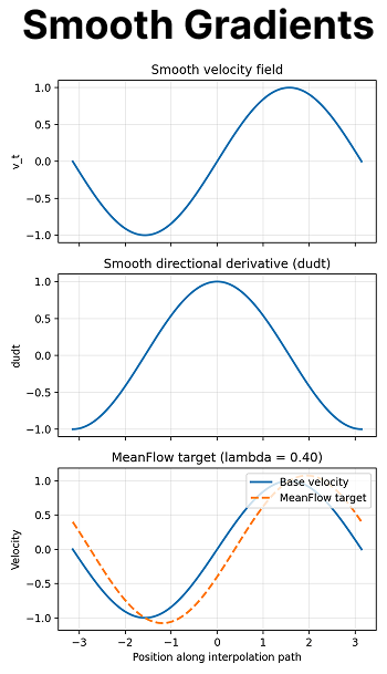
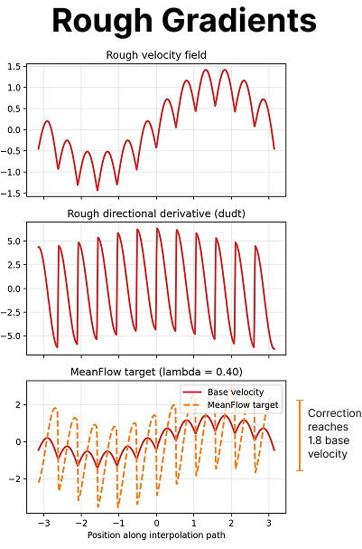
When we talk about smooth gradients we mean the network's output stays locally linear, which simply means that small nudges in the inputs produce (proportionally) small changes on the gradients.

A rough gradient would then be the opposite. Two almost identical inputs can give wildly different gradients, so the directional derivative spikes.

In both mathematics and ML (pytorch) we have what's called a Jacobian matrix. Mathematically this is:

$J = \begin{bmatrix} \frac{\partial f_1}{\partial x_1} & \frac{\partial f_1}{\partial x_2} & \cdots & \frac{\partial f_1}{\partial x_n} \\ \frac{\partial f_2}{\partial x_1} & \frac{\partial f_2}{\partial x_2} & \cdots & \frac{\partial f_2}{\partial x_n} \\ \vdots & \vdots & \ddots & \vdots \\ \frac{\partial f_m}{\partial x_1} & \frac{\partial f_m}{\partial x_2} & \cdots & \frac{\partial f_m}{\partial x_n} \end{bmatrix}$

But it might be easier to think of it in simplified pytorch terms.

Imagine we have a 10x10x3 image and a random timestep. We have a flow matching model such that: model(x, t) where x is the flattened iamge. Since this is flow matching, we get out a single value per vector, ie $x = model(x, t)$ , $x$ would be a 300 long vector.

Now, a super simple way of looking at the Jacobian matrix is thinking of doing a single forward pass with the image and timestep. We get our baseline result.

We then run a single forward step per parameter with a tiny little change. This means we do 300 forward pases (one per pixel of image) and a final one for time. Each pass we only nudge the individual parameter by a tiny amount and leave the rest constant.

In the end, we substract the resulting vector from the baseine result, divide over the tiny step and there we go, directional derivative! Then we form a matrix, our Jacobian, with our 301 (pixels + time) results (after substraction and division).

If you think about it, this matrix would tell us if we nudged each parameter, how much would the output change.

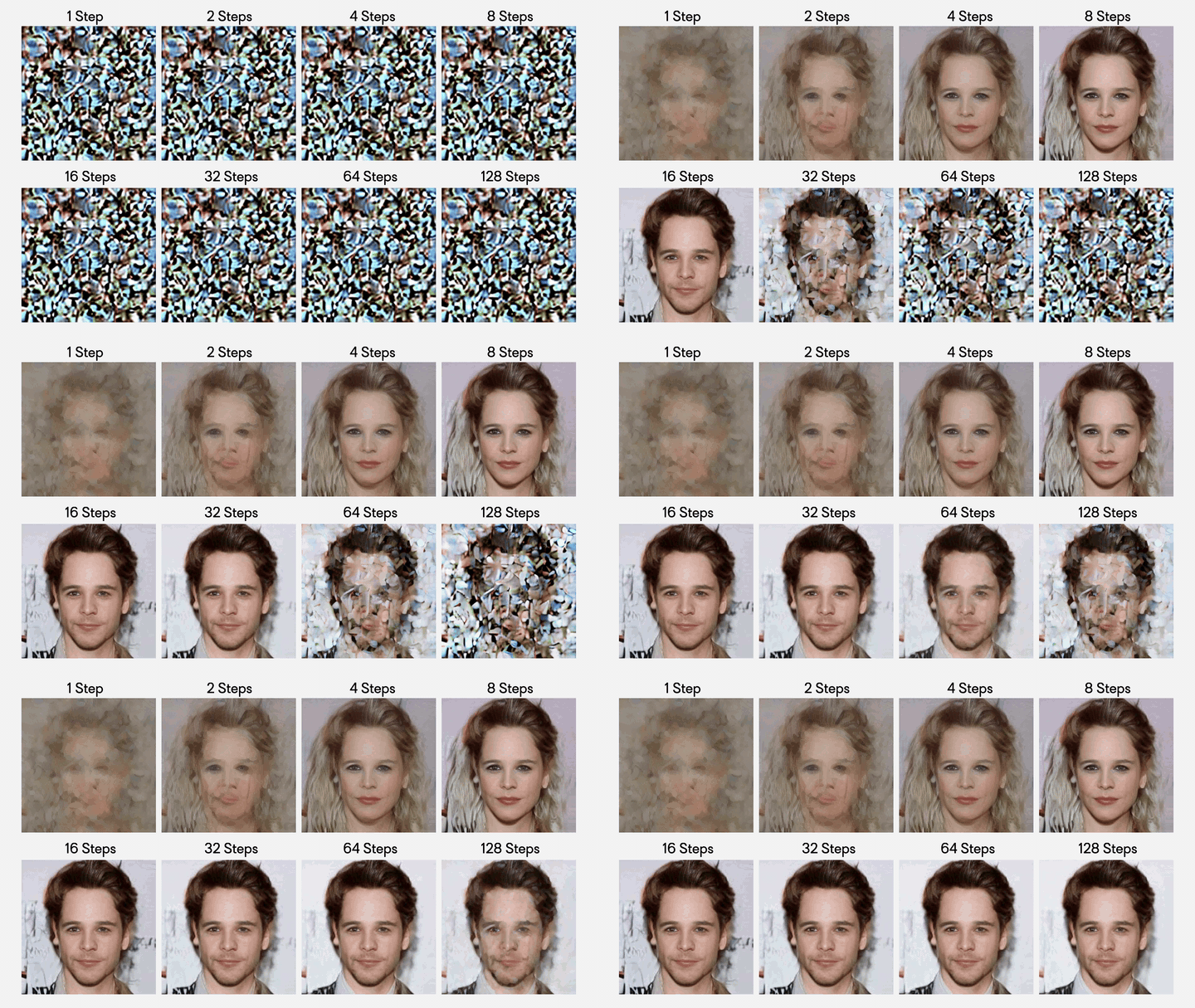
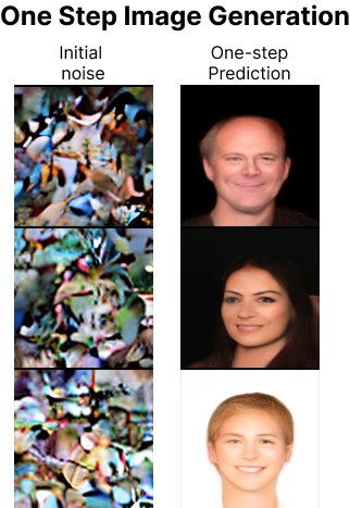
Results from a SiT-L/2 model (24 layers, 1024 hidden size, ~458M parameters) trained on CelebA (128×128) for 36,000 steps using Adam (lr=1e-4, batch size 225) on an A100 80GB (~22 hours). The training used logit-normal time sampling and 75% r≠t ratio for JVP computation.

Below are single-step samples demonstrating one-step generation without mode averaging:

MeanFlow CelebA Results

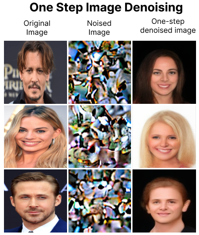
I also took some images from the internet, which were definitely not on the training set, added 75% noise and asked the model to denoise in a single step. These were the results:

MeanFlow Denoising Results

We also tested running the model for multiple steps. The results show how the model's output evolves as the number of steps increases:

MeanFlow Multi-Step Results

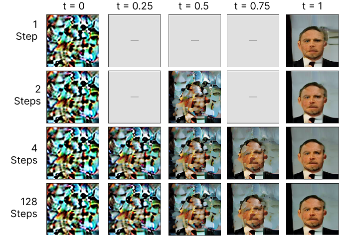
The results for one-step generation look really good, but the model uses 10x the parameters compared to Shortcut (~458M vs ~33M), which isn't a fair comparison. I initially tried training MeanFlow on a toy example but couldn't get meaningful results, then attempted using the same small diffusion transformer I'd used for Shortcut Models, but it wouldn't converge. Eventually I switched to the exact architecture from the paper (SiT-L/2, their largest model) and trained on the smaller CelebA dataset instead. Resource limits meant I couldn't retrain with a smaller model after getting this to work.

This finally worked, but training was significantly more challenging than Shortcut: longer training times, gradient instability, and overall brittle behavior. The training metrics were also particularly odd to observe; neither loss component would consistently decrease, making it difficult to identify progress. I could simply be doing something wrong though

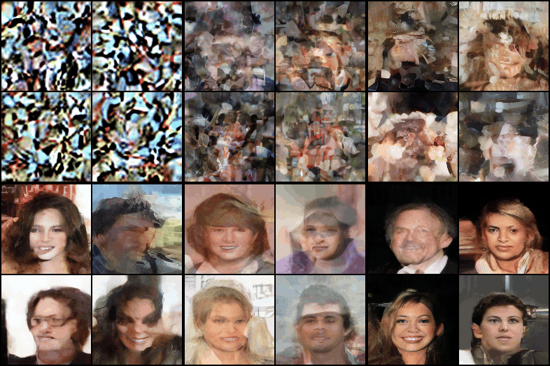
The following visualization shows what the model learned epoch by epoch. It's quite incredible to see because this is one-step sampling, mapping directly from noise to image. The model eventually finds this direct path, but the learning process resembles a painter. It starts with absolutely nothing, just random colors, then slowly fills in the image: first the background, then a rough circle with the right skin tone, then blobs where hair and eyes should go. These blobs gradually sharpen and define themselves until a coherent face emerges

MeanFlow Training Progress

Honorable Mentions

ReFlow - [Paper]

ReFlow is a simple yet supposedly effective technique that straightens the probability flow trajectories. The idea is to train a flow model, then use it to generate paired samples (noise, data), and retrain on these straighter paths.

This iterative straightening process makes few-step generation more effective by reducing the curvature of the flow trajectories. Literally making them straighter by 're-flowing'.

This is supposed to be the best FID result ever according to the numbers on the literature but the authors provide no code to replicate their results and I couldn't find anything confirming their score.

Also fundamentally I don't think that retraining the model over and over is a great idea.
CAF (Constant Acceleration Flow) - [Paper]

The fundamental idea behind CAF is to modify the standard assumption of linear paths. They introduce an idea from physics: what if we model flows with constant acceleration instead of constant velocity? I was initially happy to read this becuase I had a very similar idea, it seemed obvious to try. They also show some really good metrics.

Despite the initial excitement though, I wasn't able to get good results from these models. In some of my experiments they performed worse than even standard flow matching for multiple steps. They did perform ok on few/single step generation but the results weren't nearly as good as the two models we just presented.

Overall it's an interesting idea but I wasn't able to recreate the great results they show.

Conclusion

We explored two approaches: Shortcut Models for few-step generation and MeanFlow for single-step generation. Shortcut was significantly easier to use: a small model with stable training from start to finish. MeanFlow required a much larger model and was quite brittle (we shortly explored why, a more detailed blog might come later), but the results after one step are really good!! In general, shortcut models are great and might even replace standard flow matching in certain cases, MeanFlow is interesting despite the difficulty and still unmatched for literal single step (though they seem to lose general ability for multiple steps).

Something that I'm excited bout is few step improvements for latent space translation in world models, letting them explore action spaces more efficiently, faster inference means they could even be practical for robotics and interactive environments. Potentially for real time inference.

update They're being used in agent training: Dreamer 4 extends shortcut models to get real-time world model inference with just 4 steps instead of 64!!

The philosophical question from the intro "is single-step diffusion still diffusion?" remains open. But we're closer now. We know how to train models that generate in one step, and we've seen how they learn differently from multi-step models. The answer is somewhere in understanding what we lose/gain when we compress the iterative process. This is too long already, more on this later.

References

[1] Classical Diffusion Models Explained. YouTube Video. https://www.youtube.com/watch?v=hRi3ouF1vqY

[2] Esser, P., Kulal, S., Blattmann, A., et al. (2024). Scaling Rectified Flow Transformers for High-Resolution Image Synthesis. arXiv:2403.03206. https://arxiv.org/pdf/2403.03206

[3] Black Forest Labs. (2024). FLUX: Fast Latent Unified X-formers. arXiv:2506.15742. https://arxiv.org/pdf/2506.15742

[4] Wang, Y., et al. (2025). Wan: World-Aware Video Generation. arXiv:2503.20314. https://arxiv.org/pdf/2503.20314

[5] Pandey, K., et al. (2024). Shortcut Models for Flow Matching. arXiv:2410.12557. https://arxiv.org/pdf/2410.12557

[6] Chen, R., et al. (2025). MeanFlow: One-Step Flow Matching with Mean Velocity. arXiv:2505.13447. https://arxiv.org/pdf/2505.13447

[7] Kim, D., et al. (2024). Constant Acceleration Flow for Improved Few-Step Generation. arXiv:2411.00322. https://arxiv.org/pdf/2411.00322

[8] Liu, X., Gong, C., & Liu, Q. (2022). Flow Straight and Fast: Learning to Generate and Transfer Data with Rectified Flow. arXiv:2209.03003. https://arxiv.org/pdf/2209.03003

[9] Tau Robotics. World Models: A Survey on Latent Space Modeling. https://www.tau-robotics.com/blog/world-models#top

[10] Mehta, S., et al. (2023). Matcha-TTS: A Fast TTS Architecture with Conditional Flow Matching. arXiv:2310.16338. https://arxiv.org/pdf/2310.16338

[11] Venkatraman, S., et al. (2025). Flow Matching for Generative Modeling in Reinforcement Learning. arXiv:2505.05470. https://arxiv.org/pdf/2505.05470

[12] Chi, C., et al. (2025). Flow Matching for Robot Manipulation. arXiv:2508.11002. https://arxiv.org/pdf/2508.11002